Chapter 5 — Trigonometric Functions of Real Numbers
5.5 - More Trigonometric Graphs
§2.5 showed how to shift, reflect and stretch any function of the prototype catalog without redoing its analysis from scratch. The trigonometric functions admit the same transformations —and one more, proper to their periodicity, that no function of Chapter 2 needed.
§1. Transformations already known
Section titled “§1. Transformations already known”The vertical shift — moves the graph units upward— and the reflection about the horizontal axis — inverts each value— are particular cases of the general transformations already proved in §2.5, applied here without any adaptation: neither the periodicity nor the bounded range of and alters those proofs in any way. They are not repeated in this section.
What §2.5 could not anticipate is what happens when stretching a periodic function horizontally: for the functions of that catalog —powers, roots— stretching horizontally changed the shape of the curve, but none of them had a period that this stretching could alter. With the trigonometric functions, it does.
The vertical stretch is the simplest to treat: it does not interact with periodicity at all. It is the content of §2.
§2. Amplitude
Section titled “§2. Amplitude”Proposition. For , .
Proof. Since —§5.3 §3—, multiplying by preserves order and scales the interval: , and since attains every value of , attains every value of .
Definition. The number is called the amplitude of —or of —: half the distance between the maximum and the minimum value that the function attains.
The horizontal stretch, on the other hand, does interact with periodicity —and in a way that requires a proof of its own, not an analogy with §2.5—. It is the content of §3.
§3. Change of period
Section titled “§3. Change of period”Proposition. For , is the minimal positive period of .
Proof. That is a period: , using the periodicity of —§5.3 §4—.
That it is the minimum: suppose that is also a period, that is, for all . In particular, at : . Since , and by §5.3 §7 the only zeros of in are at , it follows that , that is, . But then, evaluating the periodicity condition at is no longer enough: it must hold for all , and in particular for it was already used; test at , where : —by the central symmetry of §5.4 §2, —, which does not coincide with . Hence does not satisfy the periodicity condition for all , a contradiction. No candidate remains in , so that is the minimal period.
Definition. The number is called the period of —or of —.
The horizontal shift —moving the graph to the left or to the right— is, on the other hand, exactly the general case already covered by §2.5, without any additional subtlety. It is the content of §4.
§4. Phase shift
Section titled “§4. Phase shift”Definition. In , the number is called the phase shift: the graph of shifted units horizontally —to the right if —, exactly according to the general transformation of §2.5.
No proof of its own is needed: it is the same horizontal transformation of §2.5, with .
Combining the four transformations —amplitude, period, phase, vertical shift— in a single expression, one obtains the general form that appears in almost any real application of these functions. It is the content of §5.
§5. The general form
Section titled “§5. The general form”has amplitude —§2—, period —§3—, phase shift —§4—, and vertical shift —§2.5—. Each parameter affects the graph independently of the other three: modifying one does not alter what the others already determined.
Worked example. Identify the amplitude, period, phase shift and vertical shift of , and graph it.
Solution. Comparing with the general form: , , , . Amplitude : the graph oscillates between and . Period : each complete oscillation occupies an interval of length , half that of . Phase shift : the graph of moved units to the right.
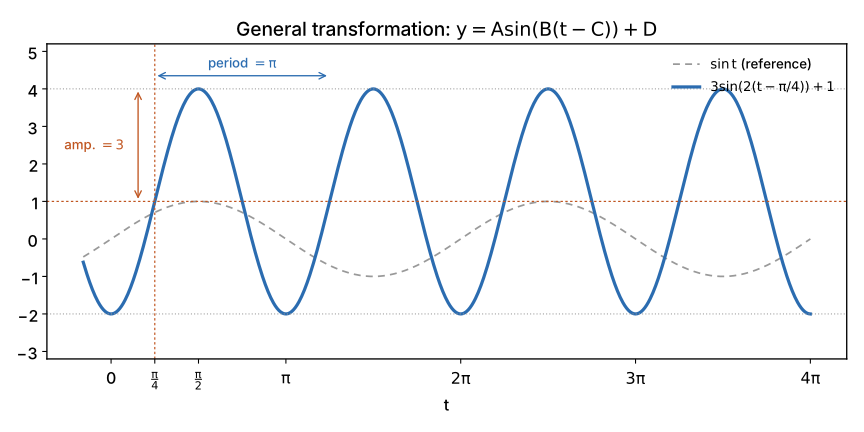 Figure 5.4 — (solid curve), compared with (dotted curve). The amplitude triples the height of the oscillation; the period is halved; the whole curve ends up shifted vertically one unit and horizontally .
The general form of this section is, precisely, the one that appears when modeling any phenomenon that oscillates with regularity. A brief example closes the section before the exercises. It is the content of §6.
§6. An applied model
Section titled “§6. An applied model”The depth of the water in a port, measured in meters above a reference level, varies with the tide in an approximately periodic way, with a complete cycle every hours, a maximum depth of meters, a minimum of meter, and the high tide occurring at in the morning.
Model. Amplitude: . Vertical shift: —the midpoint between maximum and minimum—. Period hours: by §3, . Phase: the maximum of occurs at —where the sine equals —; equating to hours and solving, with , one obtains . The resulting model:
with in hours since midnight.
§7. Worked exercises
Section titled “§7. Worked exercises”Exercise 1. Give the period of .
Solution. By §3 —applicable to by the same argument, replacing with —, the period is .
Exercise 2. Give the amplitude, the period and the vertical shift of .
Solution. —the amplitude is —, period —unchanged, since —, vertical shift . The negative sign of does not change the amplitude, but it does invert the graph —reflects it about —, according to the reflection transformation of §2.5.
Exercise 3. At which instants, according to the model of §6, is the depth of the water exactly meters?
Solution. We seek with , that is, . By §5.3 §7, this occurs when , that is, hours: at midnight, at , at , at , and so on every hours —half the period, the instants at which the tide crosses its mean level—.
§8. Close of the chapter
Section titled “§8. Close of the chapter”This chapter traveled, in five sections, a path that no elementary trigonometry course travels completely: constructing instead of taking it as known, constructing the wrapping function instead of assuming that “an angle determines a point on the circle”, and deriving each property of sine and cosine —Pythagorean identity, periodicity, parity, signs, asymptotes of their reciprocals, even the period of the tangent— from that single geometric construction, without appealing at any moment to a separate right triangle or to a memorized table of values.
The result is a family of functions as rigorously grounded as the exponential and the logarithm of Chapter 4, and with the same kind of honest limit: just as this book could not say in what precise sense the rate of change of is equal to itself —a question reserved for Calculus I—, neither could it say here how fast changes at each instant, nor why that rate turns out to be, precisely, . That connection —the heart of why the trigonometric functions are indispensable in the physics of oscillations, not only in the geometry of the triangle— will remain pending, with the same honesty, until the book reaches the derivative.
With this, Chapter 5 is closed. Chapter 6 takes up the trigonometric functions again to solve, in the inverse direction, equations and identities more general than those that this introduction could cover.
Copyright © 2026 Carlos Dagorret — Licensed under Creative Commons Attribution-NonCommercial-NoDerivatives 4.0 International (CC BY-NC-ND 4.0)