Chapter 2 — Functions
2.4 — The Catalog of Prototype Functions and Asymptotic Behavior
Before transforming a function, one needs to know the function being transformed.
The vocabulary of §2.3, with its domain, image, zeros, sign, symmetry and monotonicity, was built for any function. This section puts it to work on a few concrete functions, chosen not for their difficulty but for the opposite reason: they are the simplest of each family, and for that reason they will serve as a base, in §2.5, for building many other functions by transformation without repeating the analysis from scratch. One of them, moreover, will display a phenomenon the book mentioned only in passing in §1.9: that of a function whose values grow without bound.
§1. The elementary gallery
Section titled “§1. The elementary gallery”Six functions form the basic catalog of the chapter.
| Function | Domain | Image | Parity | Monotonicity |
|---|---|---|---|---|
| Odd | Increasing on | |||
| Even | Decreasing on , increasing on | |||
| Odd | Increasing on | |||
| Even | Decreasing on , increasing on | |||
| Neither | Increasing on | |||
| Odd | Decreasing on and on , separately |
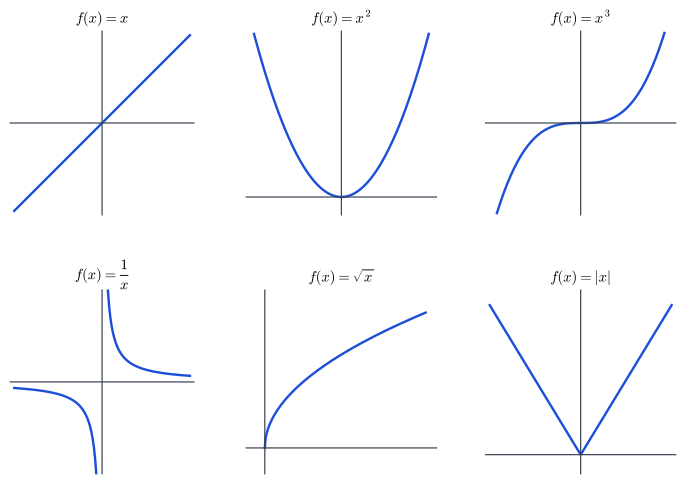
Figure 2.2 — The six prototypes of the elementary gallery.
Each row of the table is a statement that can be proved with what we already have. The domains come from §2.2: requires a nonnegative radicand and a nonzero denominator. The parities are checked as in §2.3: for example, says that is odd, and says that the absolute value is even. The monotonicity of was proved in §2.3, and that of is immediate, because for and for . The images and the remaining monotonicities are left.
For the images, we must see that each value in the column is reached and that no other value is. Every real is the cube of some real, because by §1.2 exists; the image of is . Every is the square root of , and a square root is never negative; the image of is . Every is the reciprocal of , and a reciprocal is never zero; the image of is .
For the monotonicities, the tool is again the lemma of §1.2: if , then . The function is increasing on : if , the lemma gives ; if , the lemma applied to gives , that is, ; and if , then . The function is increasing on : if and we had , the lemma would give , which is false. The function is decreasing on : if , multiplying by the positive number gives . On the argument is the same, because if and are both negative, is positive.
Two rows deserve a comment for what they anticipate.
The first is that of , which is neither even nor odd for a structural reason: its domain, , is not symmetric with respect to the origin. The comparison between and that §2.3 requires is not even possible for , and parity is ruled out beforehand.
The second is that of , whose monotonicity is declared separately on each branch, and , and not over its whole domain. This is no oversight. The function is decreasing on each branch, but it is not decreasing on : with and we have and yet . Nor is it increasing, because with and we have . The definition of monotonicity in §2.3 asks for an interval, and is not one: it lacks precisely the point that separates the two branches. What happens near that point is the topic of the rest of the section.
§2. Unbounded growth: the vertical asymptote
Section titled “§2. Unbounded growth: the vertical asymptote”Of the six functions in the catalog, five have no “forbidden” point in the middle of their domain near which something unusual might happen. The exception is , at the only point its domain excludes, . Let us ask precisely what happens to as approaches that point without being able to reach it.
The intuitive answer, ” gets larger and larger”, needs the same kind of rigor that the idea of being near received in §1.1: there, “near” was translated into the condition . Here we must translate what “becoming arbitrarily large” means.
Definition. Let be a function and such that, for every , there is some with . We say that grows without bound as tends to from the right, and we write , if
Likewise, decreases without bound as if the conclusion is , and the versions from the left, , are obtained by replacing the condition with . If any of these four situations occurs, the vertical line is called a vertical asymptote of .
The definition parallels that of a neighborhood in §1.1. There the idea was “for every margin , there is an interval where the distance to is less than that margin”; here it is “for every bound , however large, there is an interval to the right of where already exceeds it”. One measures closeness to a fixed value; the other says there is no possible fixed value, because exceeds any ceiling that is proposed.
Proposition. grows without bound as .
Proof. Let be arbitrary, and choose . If , we multiply this inequality by the positive number , which preserves its direction (§1.7), and obtain . We have proved that implies . Since was arbitrary, the definition is satisfied.
The value does not come out of nowhere: it is what one obtains by solving the inequality for , with the methods of §1.7, and choosing at the exact point where the inequality starts to hold.
§3. Approach at infinity: the horizontal asymptote
Section titled “§3. Approach at infinity: the horizontal asymptote”There is a second phenomenon at the other end of the domain of : what happens when itself grows without bound. The question is reversed with respect to the previous one, because it is no longer the variable that approaches a forbidden point, but the variable that moves away indefinitely. And the answer is reversed too: does not grow without bound, but comes closer and closer to a fixed value.
Definition. Let be a function defined for every greater than some number. We say that approaches a real as grows without bound, and we write , if
If this occurs, the horizontal line is called a horizontal asymptote of . The version for is obtained by replacing with .
The symbol is not a number: the notation is an abbreviation of ” grows without bound”, and the whole definition speaks only of real numbers and . This definition reuses unchanged the distance of the neighborhood of §1.1; the only new thing is the hypothesis that triggers it, , instead of lying in a bounded interval.
Proposition. approaches as .
Proof. Let be arbitrary, and choose . If , then , and multiplying by the positive number gives . Moreover , so that
We have proved that implies , for any .
§4. The remaining cases, by symmetry
Section titled “§4. The remaining cases, by symmetry”Two cases of the behavior of remain: what happens as and as . There is no need to repeat the arguments from scratch, because is odd, and oddness translates each case on the right into the corresponding case on the left.
If , the number satisfies . With , the proposition of §2 gives , and by oddness . Therefore decreases without bound as , and the line is a vertical asymptote from the left as well, with the sign reversed.
Likewise, if with , the number satisfies , and the proposition of §3 gives ; since , also . The line is a horizontal asymptote toward the left as well, with the same value . This is no accident: if an odd function approaches to the right, it approaches to the left, and here .
None of the other five functions in the catalog has asymptotes. Their domains exclude no interior point, and as grows or decreases without bound, their values do not settle down either: and grow without bound to the right and decrease without bound to the left, and grow without bound in both directions, and grows without bound to the right, its only unbounded end. Within this catalog, is the only one that displays both phenomena, that of an excluded point near which the function shoots off and that of a function that settles around a value as the variable moves away.
What this catalog lets us glimpse, beyond the case of , is that infinity appears in two forms that should not be confused. One is infinity as a destination: what happens to when itself moves away without bound, a question about the long run. The other is infinity as a local symptom: a function defined near a point, except at the point itself, whose values shoot off as approaches it. In neither does “reach” infinity: no and no , however large, exhaust the definition. Both are statements about every finite threshold.
And at bottom they are the same phenomenon. Both are particular cases of a single notion, that of limit, which this section built twice without naming it, once with and , once with and . Naming it now changes no definition and no proof: what we defined are, exactly, the limits ” tends to as ” and ” tends to as ”, together with the variants we obtained by symmetry. What lies outside this book, and properly belongs to Calculus, is the general theory: the limit as approaches from both sides at once, the rules that allow one to compute the limit of a sum, a product or a quotient from the limits of the parts without repeating each time an argument like those of this section, and the notion of continuity that rests on all of it. This book built the concept in the cases it needed; systematizing it is a different work.
With the gallery of prototypes analyzed, including its behavior at the edges of the domain, the chapter has the raw material for the next step: transforming these six functions, shifting, stretching and reflecting them, to obtain a much larger family without repeating the analysis from scratch. That is the topic of the next section.
Copyright © 2026 Carlos Dagorret — Licensed under Creative Commons Attribution-NonCommercial-NoDerivatives 4.0 International (CC BY-NC-ND 4.0)