Chapter 2 — Functions
2.8 — Optimization and Extreme Values: Local Behavior
Before asking how the optimum is computed, one must ask what it means, precisely, for a value to be the best.
The properties studied so far describe a function as a whole, or at least on long stretches of its domain: monotonicity, symmetry, asymptotic behavior. This section deals instead with isolated points: those at which a function reaches its highest or lowest value, whether on its whole domain or only near the point. It is the first section of the chapter devoted to the local behavior of a function, and also the one that must be clearest about how far one can go without the tools of Calculus, which this book does not include.
§1. Absolute and relative extrema
Section titled “§1. Absolute and relative extrema”Definition. Let be a function and . We say that has an absolute maximum at if for all ; in that case, is the maximum value of . Likewise, has an absolute minimum at if for all .
The word “absolute” indicates that the comparison is made against the whole domain. There is a more modest notion, which only requires being the best value near the point, and which uses the neighborhood of §1.1, the same one that appeared in §2.4.
Definition. Let be a function and . We say that has a relative maximum, or local maximum, at if there exists such that
and a relative minimum at if for all in that same set. Maxima and minima are called, together, extrema.
With this definition, every absolute extremum is also relative: if is the largest value on the whole domain, in particular it is the largest within any neighborhood of . The converse is false: a relative maximum may be the largest value only near , with higher values elsewhere in the domain.
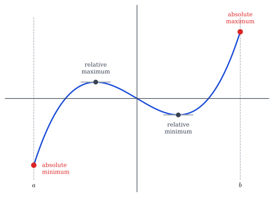
Figure 2.6 — Interior relative extrema (a local maximum and a local minimum) compared with the absolute extrema, reached here at the endpoints and of the interval. The curve is schematic: it illustrates the vocabulary of this definition, not the result of the tools of this section.
§2. Extrema of quadratic functions: the vertex
Section titled “§2. Extrema of quadratic functions: the vertex”The most accessible case, and the most frequent one in applications at this level, is that of a quadratic function , with . Section 1.3 completed the square to factor the trinomial; the same computation, read with another purpose, gives the extremum of the function.
Proposition. Let , with , and . If , has an absolute minimum at , with value . If , it has at the same point an absolute maximum with that same value.
Proof. Completing the square as in §1.3,
If , the term is the product of a positive number and a square, so it is never negative, and it equals exactly when . Therefore for every , with equality only at that point. If , the same term is never positive, the inequality is reversed and an absolute maximum is obtained.
The sign of decides whether the parabola opens upward, and then its lowest point is an absolute minimum, or downward, with an absolute maximum. The point of the graph is called the vertex.
Example. Among all rectangles with perimeter , which has the largest area? If one side measures , the other measures , with , and the area is . Here , and the proposition gives an absolute maximum at , with area . The optimal rectangle is the square with side . The vertex falls within the domain the problem allows, the interval , and that is why it is the answer.
That last check is not a detail. In the geometric problem of §1.6, the area was . With , the proposition gives an absolute minimum at , with value . The result is correct as a statement about the formula, but it says nothing about the problem: a width cannot be negative, nor can an area. As in §1.6, the extremum of a formula matters only if it falls within the domain the problem allows, here , where is increasing and has no extremum at all.
§3. Extrema through monotonicity
Section titled “§3. Extrema through monotonicity”When a function is not quadratic but its monotonicity is known, from the analysis of §2.3 or because it comes from a prototype transformed according to §2.5, its extrema on a closed interval follow from the definition of monotonicity.
Proposition. If is increasing on , then its absolute minimum on that interval is at and its absolute maximum at . If is decreasing on , the roles are reversed.
Proof. Suppose is increasing on and let . If , then ; if , the definition of §2.3 gives . In both cases, . Likewise, . Therefore for every . The decreasing case is analogous.
Example. The function is increasing on (§2.4). Restricted to the interval , its absolute minimum is and its absolute maximum is , with no computation beyond evaluating at the endpoints of the interval.
§4. The inequality between the means and extrema under a constraint
Section titled “§4. The inequality between the means and extrema under a constraint”There is a kind of problem that does not fit the previous cases: one in which two quantities are linked by a constraint, for example a fixed sum, and one seeks the extremum of a third quantity built from them, for example their product. A classical inequality solves many of these problems without reducing them to a function of a single variable.
Proposition (inequality between the arithmetic and geometric means). For ,
with equality if and only if .
Proof. Since , the roots and exist (§1.2), and since no real square is negative (§1.3),
where we used (§1.2). Dividing by gives the inequality. Equality holds if and only if , that is, if , and by the uniqueness of the root, if .
The number is the arithmetic mean of and , and their geometric mean. The inequality is usually abbreviated AM-GM.
Example. Let us generalize the example of §2: among all rectangles with perimeter , which has the largest area? Let be the sides. The fixed perimeter gives , that is, . By the inequality,
where in the last step we squared two nonnegative numbers, which preserves the direction by the lemma of §1.2. The area never exceeds , and by the equality condition that value is reached exactly when : the optimal rectangle is the square. With we recover the result of §2. The constraint and the quantity to be maximized were combined directly, without building a function of a single variable.
§5. How far these tools go
Section titled “§5. How far these tools go”The three tools of this section, the vertex of the parabola, monotonicity and the AM-GM inequality, solve a significant share of the optimization problems at this level, but they do not form a general method. None of the three says where the relative extrema of, for example, are: it is not quadratic, its monotonicity changes direction at points these tools do not allow one to locate without knowing them beforehand, and it does not have the form of a fixed sum with a variable product. Determining the extrema of arbitrary functions, without depending on their having one of these particular structures, is one of the problems that motivate differential Calculus, with a tool, the derivative, capable of locating relative extrema without knowing the form of the function in advance. What has been developed here is not a general method disguised as a particular case, but what the title announces: an introduction to local behavior with the means available in this book.
The search for an extremum, the largest, the smallest, the most efficient, is not a concern exclusive to this section or to mathematics. A ray of light travels between two points along the path that minimizes the travel time; a soap bubble takes, among all the shapes enclosing a given volume, the one with the least surface; an ant colony builds routes that approach, without conscious computation, a path of minimal length. That nature seems to solve optimization problems again and again, without equations or inequalities, is one of the most persistent coincidences between mathematical structure and the behavior of the world. The question remains open whether that coincidence reveals something deep about how the world is made, or whether it is mathematics that finds economy everywhere because those are, of all possible structures, the simplest to describe.
With the extrema made precise, including the limits of what can be achieved without Calculus, the chapter completes its technical journey: from the function as a set of pairs to its domain, its global behavior, its prototypes and transformations, its algebra and composition, its reversibility and this first contact with optimization. The next section closes the chapter with a historical look at the very concept of function.
Copyright © 2026 Carlos Dagorret — Licensed under Creative Commons Attribution-NonCommercial-NoDerivatives 4.0 International (CC BY-NC-ND 4.0)