Chapter 4 — Exponential and Logarithmic Functions
4.3 - Logarithmic Functions
Every injective function keeps, in its own behavior, the possibility of undoing itself. The exponential has already shown itself to be one; all that remains is to claim that possibility.
§4.1 proved, for with , much more than was needed at the time: not only that is strictly monotone (§9, section 4.1), from which its injectivity follows, but also that its range is exactly (§10, section 4.1), with nothing missing. Those two pieces, taken together, are exactly what §2.7 required to guarantee the existence of an inverse function: injectivity for the uniqueness of the preimage, surjectivity, onto the correct codomain, for its existence. Nothing new needs to be proved to obtain the inverse; all that is needed is to recognize that the conditions are already given.
§1. Bijectivity of aˣ and existence of the inverse
Section titled “§1. Bijectivity of aˣ and existence of the inverse”Fix , , and consider , , with the codomain restricted exactly to its range, as already proved.
Proposition. is bijective.
Proof. Injectivity: Corollary of §9, section 4.1. Surjectivity: since the codomain was fixed equal to the range, , §10, section 4.1, guarantees that every element of the codomain is attained.
By §2.7 §3, every bijective function admits an inverse, unique, characterized by the identities and . Applied here:
Definition. The inverse function of is called the logarithmic function with base , and is denoted . That is: for , is the unique such that .
With defined as an inverse, it is time to make explicit the two identities that characterize it completely, and which in practice are the most direct computational tool. That is the content of §2.
§2. Inversion identities
Section titled “§2. Inversion identities”By the general characterization of every inverse function, §2.7 §3, applied here to and , we have, without additional proof, the two identities:
The first says that applying the logarithm after the exponential returns the original exponent; the second, that applying the exponential after the logarithm returns the original number. Neither is a new property of the logarithm: it is, literally, the definition of inverse, §2.7 §3, specialized to this pair of functions.
With the function and its characteristic identities defined, it is time to specify its sets of definition and arrival, which, since is an inverse, require no new computation. That is the content of §3.
§3. Domain and range
Section titled “§3. Domain and range”Proposition. and .
Proof. By §2.7 §4, for every bijective function , and ; domain and image are exchanged completely. Applied to , with and , §10, section 4.1, we obtain immediately and .
It is worth pausing on what this means in practice: is not defined for , since neither zero nor any negative is ever attained by , according to the range of the exponential itself, while, in the other direction, every real number, however large or small, is the logarithm of some .
Domain and range were resolved by direct inheritance. Monotonicity, on the other hand, requires its own proof, since §2.7 did not prove it in general for every inverse, and is the content of §4.
§4. Strict monotonicity
Section titled “§4. Strict monotonicity”Proposition. If , is strictly increasing on . If , is strictly decreasing on .
Proof. Let with , and let , , so that and , by the definition of §1.
Case . Suppose, for contradiction, . Since is strictly increasing for , §9, section 4.1, in particular it is nondecreasing: implies , that is, , contradicting . Hence , that is, .
Case . Suppose, for contradiction, . Since is strictly decreasing for , §9, section 4.1, in particular it is nonincreasing: implies , that is, , contradicting . Hence , that is, .
With domain, range and monotonicity already established, what remains are the distinguished values of the logarithm, its behavior at the ends of the domain, its graph, and the block of exercises and close.
§5. Distinguished values
Section titled “§5. Distinguished values”Proposition. and .
Proof. By the rational consistency of §6 (or §7) of section 4.1, . By the Definition of §1, is the unique real with ; since , that unique real is . Likewise, , a trivial particular case of exponentiation, so that is the unique real with , and that real is .
It remains to describe what happens with at the ends of its domain: near , where the domain ends but does not include that point, and when grows without bound. That behavior is, exactly, the mirror of §11 of section 4.1, with the roles of domain and range exchanged.
§6. Asymptotic behavior
Section titled “§6. Asymptotic behavior”Proposition (case ). For every there exists such that . Moreover, for every there exists such that .
Proof. Let . Suppose and, for contradiction, . Since is nondecreasing for , §9, section 4.1, implies , that is, , contradicting . Hence .
Let . Suppose and, for contradiction, . By the same monotonicity, , that is, , contradicting . Hence .
The line is, then, a vertical asymptote of when : as approaches from the right, decreases without bound. And grows without bound as , with no horizontal asymptote whatsoever.
Proposition (case ). For every there exists such that . Moreover, for every there exists such that .
Proof. Analogous to the previous one, using that is nonincreasing for , §9, section 4.1: with , if and , nonincreasing monotonicity gives , that is , a contradiction; hence . With , if and , nonincreasing monotonicity gives , that is , a contradiction; hence .
In this second case, the line is still a vertical asymptote, but with inverted sign: grows without bound as , and decreases without bound as , exactly the mirror of the behavior of with , which decreased toward instead of growing.
With domain, range, monotonicity and asymptotics already complete, the graph of requires no new analysis: it is obtained, geometrically, from the already known graph of . That is the content of §7.
§7. Graph and symmetry about y = x
Section titled “§7. Graph and symmetry about y = x”By §2.7 §4, the graph of every inverse function is the reflection of the graph of the original function about the line . Applied here: is, without further computation, the reflection of about that diagonal. Each feature already proved translates geometrically without an additional word: the horizontal asymptote of is reflected into the vertical asymptote of ; the point , common to every exponential, is reflected into the point , common to every logarithm, exactly what §5 asserted; and monotonicity is preserved in the same direction, because a reflection about does not invert whether a curve rises or falls from left to right.
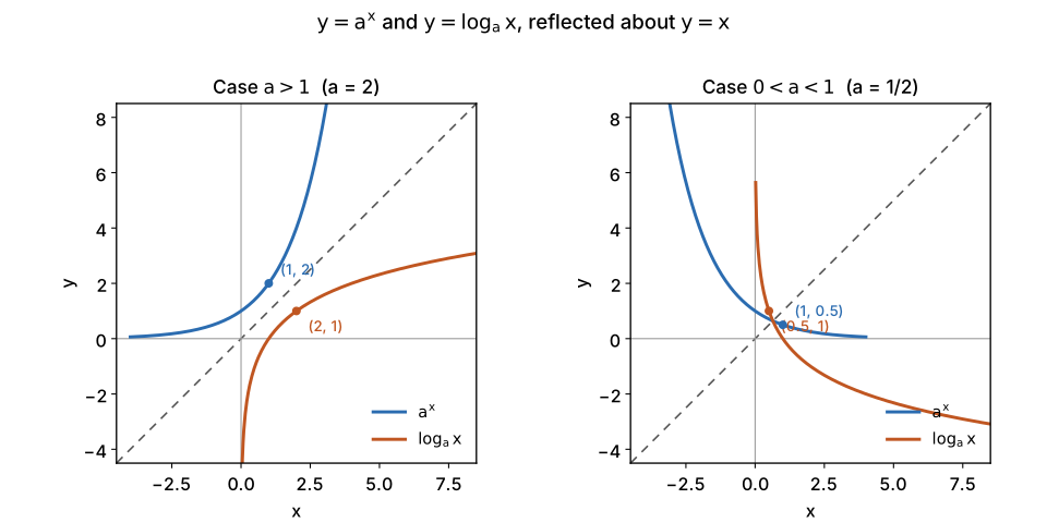 Figure 4.1 — and , reflected about , for (left, ) and (right, ). In both cases, the point corresponds to , the same type of correspondence as Figure 2.5 of §2.7 §4, applied here to a pair of curves instead of to two lines.
What remains, to close the section, is to exercise the handling of the inversion identities and of the monotonicity just proved, and a brief reflection on what the logarithm makes possible for the next section. That is the content of §8.
§8. Worked exercises and close
Section titled “§8. Worked exercises and close”Exercise 1. Compute .
Solution. , so that, by the identity of §2 with , .
Exercise 2. Solve .
Solution. By the Definition of §1, means . Hence .
Exercise 3. Solve the inequality , specifying the domain.
Solution. The domain requires , §3. Since , is strictly increasing (§4), so that , Exercise 1, is equivalent, by strict monotonicity, to . Combining with the domain, the solution is .
Exercise 4. Simplify .
Solution. By the homomorphism of §8, section 4.1, valid for any pair of reals in the exponent, and are such, . By the inversion identity of §2, each factor simplifies separately: and . Hence .
It is worth noting what was not used: at no moment was it necessary to write as the logarithm of a product; that equivalence, , is precisely the first law that section 4.4 will prove. What this exercise resolves is the opposite direction: what happens when the sum of two logarithms appears in the exponent, not inside another logarithm.
With this, the logarithm is completely constructed from a single idea, that the exponential, being bijective, can be undone, and from a single source of new results, monotonicity and asymptotics, both obtained by contradiction from what the exponential already guaranteed. There was, in this section, no construction from scratch: everything rested on §2.7, written chapters ago without yet thinking of the exponential, and on §4.1, written this very week thinking exactly of this moment. That both fit together without friction is no coincidence: it is the kind of economy the book has pursued since the first chapter, and which only becomes visible when a distant piece fits, without adjustments, into a place that did not know it was awaited.
With section 4.3 closed, §4.4 takes up the homomorphism of the exponential, §8 of section 4.1, to translate it, term by term, into the laws of logarithms: product into sum, quotient into difference, power into product.
Copyright © 2026 Carlos Dagorret — Licensed under Creative Commons Attribution-NonCommercial-NoDerivatives 4.0 International (CC BY-NC-ND 4.0)