Chapter 1 — Fundamental Concepts
1.1 — The Real Numbers
Every exact science begins by naming what it is going to speak about.
Every mathematical study needs two things: objects to work with and precise rules for operating on them. In this book, which runs from elementary algebra to the threshold of Calculus, the fundamental object is the real number, and the set of all real numbers is denoted .
This section establishes what is made of and which laws govern its operations. We will proceed in layers. Each number set arises from an operation that the previous one could not carry out, and in this way we will reach the real line with its addition, its multiplication, its order and its notion of distance. What is established here will be used throughout the rest of the book without being justified again.
§1. The natural numbers
Section titled “§1. The natural numbers”The first numbers we use are the ones that serve for counting. They form the set of natural numbers, denoted . We can describe it by listing its elements between braces, separated by commas:
The ellipsis is not decoration. It indicates that the list continues without end, following the same pattern, so that is an infinite set. Nor does the sign express an equality between numbers here; it expresses an equality between sets: it says that the set we call is exactly the one on the right. What “following the same pattern” means rigorously is a harder question than it seems. We answer it in §10.1, where the natural numbers are defined without an ellipsis.
Note. We follow the usual convention of algebra and analysis: zero is not a natural number. In other areas, such as logic or computer science, it is convenient to include it, and one then writes to distinguish the two sets. In this book always starts at .
§2. The integers
Section titled “§2. The integers”With the natural numbers we can add and multiply without leaving the set, but we cannot always subtract: is not a natural number. For subtraction to be always possible, we must add zero and the negative numbers. This extension came late in history and met resistance. Negative numbers were first used to keep track of debts, and centuries passed before they were accepted as numbers in their own right.
Adding to the natural numbers zero and the opposite of each natural number, we obtain the set of integers, denoted , from the German Zahlen, “numbers”. Listing its elements,
and, if we want to highlight its structure,
where are the positive integers, which coincide exactly with , and the negative integers. The symbol is read “union”: an element belongs to if it belongs to , to , or to both. The expression denotes the set whose only element is zero. It should not be confused with the number : we can think of as a box that contains zero. The box has one element; zero is that element.
§3. The rational numbers
Section titled “§3. The rational numbers”In subtraction no longer poses a problem, but division does: is not an integer. Sharing a quantity into equal parts, or measuring a length with a unit that does not fit a whole number of times, forces us to introduce fractions.
A rational number is a number that can be written as a quotient of two integers. The set of rational numbers is denoted , for quotient, and we define it in set-builder notation:
Set-builder notation does not list the elements; it describes them by the property they satisfy. The vertical bar is read “such that” and introduces that property. The symbol indicates membership: "" is read ” belongs to ”. The symbol negates equality. The whole expression is thus read “the set of fractions such that and are integers and is different from zero”.
The condition is indispensable: it excludes division by zero, which is not defined. Note also that different fractions can represent the same number, such as and . The criterion for deciding when two fractions are equal appears in part 6 of this section.
§4. The irrational numbers
Section titled “§4. The irrational numbers”Between any two rational numbers there is always another, their average for instance, so it might seem that fractions already fill the line. They do not. Greek mathematicians discovered that the diagonal of a square of side cannot be measured by any fraction of that side. The discovery was so disturbing that tradition surrounded it with legends, and it forced the admission that there are lengths that are not quotients of integers.
Before giving the definition, a remark on the order in which we present things. So far we have used only intuitively, as the complete number line. Its definition as a set comes in the next part, and that definition relies in turn on the irrational numbers. There is no vicious circle here, only a choice of order. First we characterize the irrational numbers by a property of their own, which does not require to have been defined. Then, once is established, we also describe them as a part of .
An irrational number is a real number that cannot be written as a quotient of integers. Equivalently, it is a number whose decimal expansion is neither finite nor periodic. That the two descriptions agree, that is, that the rational numbers are exactly the numbers with a finite or periodic decimal expansion, is proved in §10.4. The set of irrational numbers is denoted , or also , the complement of . Once is available, we can write it as follows:
The symbol negates membership. The symbol denotes set difference: consists of the elements of that do not belong to . The formula is read “the irrational numbers are the real numbers that are not rational”.
Saying that irrational numbers exist is not enough; we must exhibit one. The proof that follows is one of the oldest in mathematics, and it is also the first in this book.
Proposition. There is no rational number whose square is .
Proof. Suppose, for the sake of contradiction, that there is a rational number with . Since , we may assume that is positive and write it as , with and positive integers. Every fraction can be simplified, by dividing numerator and denominator by their common factors, until none remain. We therefore choose and with no common factors. From we obtain
The last equality says that is even. This forces to be even. Indeed, if were odd, we would have for some integer , and then would be odd. We therefore write with an integer, and substitute:
Now it is that turns out to be even, and by the same argument is even as well. But we had chosen and with no common factors, and we have just seen that both are divisible by . The contradiction comes solely from having assumed that existed. Therefore no rational number has a square equal to .
The proposition says that if there is a positive real number whose square is , the number we write and which measures the diagonal of the square of side , then that number is irrational: . That such a number exists in is not obvious, and part 9 of this section shows where it comes from. The method of the proof, assuming the opposite of what we want to prove until we reach an absurdity, is called reductio ad absurdum, or proof by contradiction, and we will use it many times.
§5. The real numbers
Section titled “§5. The real numbers”We now bring the two families together. The set of real numbers is the union of the rational and the irrational numbers:
The union is disjoint: no number is both rational and irrational, which is written . The symbol is read “intersection” and designates the elements common to two sets. The symbol designates the empty set, the only set with no elements. Two sets whose intersection is empty are called disjoint.
The sets we have built are thus linked in a chain, each contained in the next:
The symbol is read “is contained in”. The irrational numbers occupy exactly what leaves free inside .
The most important question remains open: why are the irrational numbers needed? What exactly does lack? The answer, the property that distinguishes from , is developed in part 9 of this section.
§6. The algebraic properties and the order of ℝ
Section titled “§6. The algebraic properties and the order of ℝ”On there are two operations, addition and multiplication. We will not justify their properties from something more elementary: we take them as a starting point. They are axioms, and the algebra of the whole book is deduced from them.
Both operations are commutative: the order of the terms or of the factors does not change the result.
Both are also associative, which allows us to write sums and products of three or more terms without indicating how they are grouped:
Distributivity is the property that links the two operations. Multiplying a sum by a number is the same as multiplying each term and adding the products:
Each operation has an identity element, which leaves unchanged whatever it operates on, and each number has an inverse, which undoes the operation. Zero is the identity for addition, , and every real number has an opposite with . With it we define subtraction, . One is the identity for multiplication, , and every real number has a multiplicative inverse with . With it we define division, , provided . It is also assumed that . The symbol is read “is defined as”.
The opposite of each number is unique. If and , then
using the identity, associativity and commutativity. In the same way one proves that the multiplicative inverse is unique.
Signs. The rules of signs are not conventions to be memorized: they are deduced from the axioms. First, for every . Indeed, by distributivity, , and adding the opposite of to both sides leaves . Second, , because
and the opposite of is unique. Third, . By the previous rule with , the product is the opposite of , and that opposite is , because . From these three rules, together with commutativity and associativity, the complete table follows:
For example, . The others are proved in the same way, and it is worth doing so as an exercise. “Minus times minus is plus” is thus a consequence of distributivity and of the uniqueness of the opposite.
Fractions. For we write . The rules for fractions are also deduced from the axioms. Assuming all denominators are nonzero, and also in the division,
When two fractions have the same denominator, their sum is distributivity applied to the factor :
When the denominators are different, we multiply each fraction by a fraction equal to , or , to bring them to a common denominator, and apply the previous rule:
In calculations it is convenient to use the least common multiple of the denominators as the common denominator. It is obtained by factoring each denominator into primes and taking each factor with its largest exponent, and this keeps the numbers smaller. Finally, if we may cancel a common factor, , and two fractions are equal exactly when their cross products agree: . The symbol is read “if and only if”. This shows, for example, that , because .
Order. Real numbers are not only added and multiplied: they are also compared. Order is governed by a second group of axioms. There is a subset of , that of the positive numbers, with two properties. The first is trichotomy: for each real number , exactly one of the statements ” is positive”, "" and ” is positive” holds. The second is that the sum and the product of two positive numbers are positive. We write when is positive, and we define , read ” is less than ”, as . The expression means or .
From these axioms come the rules for working with inequalities. If and , then , because is a sum of positive numbers. If , then for any , because the difference is still . If and , then , because is a product of positive numbers. On the other hand, if , the inequality is reversed, , because is positive. Finally, the square of every nonzero real number is positive: if it is a product of positive numbers, and if , then . In particular . Section 1.7 develops these rules.
§7. Sets and intervals
Section titled “§7. Sets and intervals”We have already used , , and in building . It is now worth fixing their general definitions. Given two sets and ,
The union gathers what is in at least one of the two; the intersection keeps only what they share; the difference removes from what is in . When , the sets are disjoint.
One kind of subset of appears constantly: the interval, made up of all the real numbers between two endpoints . The notation indicates with parentheses and brackets whether each endpoint is included or not.
| Notation | Set | Endpoints |
|---|---|---|
| both excluded (open interval) | ||
| both included (closed interval) | ||
| includes , excludes | ||
| excludes , includes |
When the interval has no end on one side, the symbol , read “infinity”, is used, and always with a parenthesis. Infinity is not a real number, so there is nothing to include:
For example, is the set of with . The extreme case, , is all of .
§8. Absolute value and distance
Section titled “§8. Absolute value and distance”On the line, and are at the same distance from zero, one on each side. The absolute value measures that distance while forgetting the side. The absolute value of a real number is denoted and is defined by cases:
If is nonnegative, its absolute value is itself. If it is negative, it is its opposite, which is positive by trichotomy. In both cases , as befits a distance.
Four properties follow from the definition:
The first three are checked by separating cases according to the signs of and . For example, if and , then and ; the other cases are analogous. The fourth, for a natural exponent , results from applying the second repeatedly. The first says that a number and its opposite are equidistant from the origin; the others, that the absolute value respects products, quotients and powers.
A fifth property deserves a place of its own, because the rest of the book relies on it again and again: the triangle inequality,
To prove it we use a translation that will appear everywhere. If , then
Indeed, if , the condition is , and holds anyway. If , the condition is , that is, , and holds anyway. The same argument works with strict inequalities: .
Proof of the triangle inequality. By the previous equivalence with and with , we have and . Adding term by term,
and the equivalence, now read from right to left with , gives .
The absolute value of a sum never exceeds the sum of the absolute values. Equality holds when and have the same sign, or one of them is zero, and strict inequality when they have opposite signs, because then they partly cancel. This inequality, modest in appearance, is the central tool for bounding sums and differences, and it reappears in the study of limits and approximations.
With the absolute value we define the distance between any two points of the line. Given ,
Since and are opposites, the first property gives : the distance does not depend on the order in which we name the points.
Finally, a translation between inequalities and geometry that we will use constantly. Let be a positive number; the Greek letter is read “epsilon” and usually designates a small quantity. The inequality says that is less than away from . By the equivalence with strict inequalities, this means , that is, . The inequality therefore describes the open interval centered at :
This interval is called the neighborhood of of radius , and the notation recalls the word “ball”. It looks like a minor detail, but it is the language in which we will later say precisely what it means for one point to come as close as we like to another.
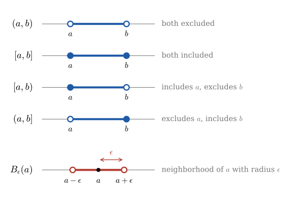
Figure 1.1 — The four types of interval and the neighborhood just defined.
§9. Completeness of ℝ: bounds, supremum and the axiom that distinguishes it from ℚ
Section titled “§9. Completeness of ℝ: bounds, supremum and the axiom that distinguishes it from ℚ”Let us return to the question left open in part 5 of this section: what does lack in order to be ? The usual picture says that is full of holes and that the irrational numbers fill them. The picture is correct, but it misleads if taken literally, because the rational numbers are not separated from one another. Between two rational numbers there is always another, their average , and repeating the argument gives infinitely many. This property is called density. The hole in does not lie in the distance between its points, but in something subtler: there are sets of rational numbers that do not extend without limit and yet have no exact rational “ceiling”. To say this precisely we need three definitions.
Bounds. Let be nonempty; the symbol is read “is a subset of”. A number is an upper bound of if no element of exceeds it, that is, if for every . If some upper bound exists, we say that is bounded above. Symmetrically, is a lower bound of if for every , and is bounded below if it has one. An upper bound need not belong to , and if has one, it has infinitely many, because every number greater than an upper bound is also one.
Supremum. Among all the upper bounds of we are interested in the tightest. The supremum of , written , is the upper bound of that is less than or equal to every other upper bound of . There is an equivalent way of saying this, which is the one most used in proofs: if and only if is an upper bound of and, for every , there is some with .
Let us see why the two formulations say the same thing. If is the least upper bound and , the number is less than and is therefore not an upper bound, so some exceeds it. Conversely, suppose that is an upper bound with that property and let . With there is with , so is not an upper bound. No upper bound is less than , and is the least.
When belongs to , it is called the maximum of . But a set can have a supremum without having a maximum: the interval has supremum , which does not belong to it. The number is an upper bound, and given , the larger of the numbers and belongs to the interval and exceeds . The symmetric notion, the greatest of the lower bounds, is called the infimum and is written .
With this vocabulary we state the property that separates from .
Supremum axiom (completeness of ). Every nonempty subset of that is bounded above has a supremum in .
This statement is not deduced from the algebraic and order axioms of part 6. It is added to them as one more axiom, as fundamental as commutativity. What we can prove is that does not have this property: there are nonempty subsets of , bounded above, with no rational supremum. That is exactly the hole.
Proposition. The set is nonempty and bounded above, but has no supremum in .
Proof. is nonempty, because . It is bounded above by : if we had , then , and would not be in .
We will use a fact about positive numbers: if , then , because multiplying by and by gives . Consequently, if and , then .
Now suppose, for the sake of contradiction, that has a rational supremum . Since , we have . By the proposition of part 4, is impossible, so two cases remain, and in each one we reach a contradiction.
Case . We will find an element of greater than , which prevents from being an upper bound. Let
which is rational and positive, because . Since , the numerator satisfies and the denominator satisfies , so that . Multiplying by we get , and then
The number is rational, positive, and its square is less than : it belongs to and is greater than . Hence is not an upper bound, a contradiction.
Case . We will find an upper bound of less than , which prevents from being the least. Let
which is rational and positive, and less than because it is obtained by subtracting a positive quantity from . Its square exceeds :
Now every satisfies , and since and are positive, the previous fact gives . Thus is an upper bound of less than , another contradiction.
Both cases lead to an absurdity, so has no supremum in .
In , on the other hand, the supremum axiom guarantees that has a supremum. And the same two-case reasoning, applied now to the set of positive real numbers whose square is less than , proves something more important: that there is a positive real number whose square is exactly . In §1.2 we carry out that proof for roots of any index. That number is , and it exists in precisely because satisfies the supremum axiom.
That is the underlying reason why the irrational numbers are needed. They are not there to complete a list of numbers that were “missing”, but so that every bounded set has, without exception, an exact ceiling. Without them, the line would have gaps in places as concrete as the diagonal of a square.
Copyright © 2026 Carlos Dagorret — Licensed under Creative Commons Attribution-NonCommercial-NoDerivatives 4.0 International (CC BY-NC-ND 4.0)