Chapter 2 — Functions
2.7 — Injectivity, Reversibility and the Inverse Function
Every function goes from cause to effect; only some also allow one to return from effect to cause.
The composition of §2.6 chained the output of one function to the input of another. This section studies a related question: given a function , is there another one that exactly undoes what did? Not every function allows it, and specifying when it does requires returning, with more care, to the codomain and the image of §2.1.
§1. Injectivity and the horizontal line test
Section titled “§1. Injectivity and the horizontal line test”Definition. A function is injective, or one-to-one, if distinct elements of the domain always correspond to distinct values:
An equivalent form, and almost always a more convenient one, is the contrapositive: . The contrapositive of an implication “if , then ” is “if not , then not ”, and it says exactly the same thing. Both forms express that no value of is reached more than once, but the second starts from an equality, which is easier to compute with.
Just as the uniqueness of §2.1 was translated into the vertical line test of §2.3, injectivity has an analogous translation on the other axis.
Proposition (horizontal line test). A function is injective if and only if each horizontal line meets in at most one point.
Proof. That the line meets in two distinct points means that there are with , which is exactly the negation of injectivity. Therefore is injective if and only if no horizontal line meets the graph in two or more points.
The parallel with §2.3 is no accident. The vertical line checked a condition on the domain: that each have a single . The horizontal line checks a condition on the image: that each reached be reached by a single . It is the same question of uniqueness, posed on different axes.
A frequent source of injectivity is the monotonicity of §2.3.
Proposition. If is increasing or decreasing on its domain, which is an interval, then is injective.
Proof. Let be in the domain; we may assume . If is increasing, , and if it is decreasing, . In both cases, .
Examples. The function is injective, because it is increasing on (§2.4). On the other hand, is not: , and on the graph, the horizontal line meets the parabola in two points. The converse of the proposition is false: is injective, because implies , but it is not monotonic on its domain, as we saw in §2.4.
§2. Surjectivity, bijectivity and the codomain
Section titled “§2. Surjectivity, bijectivity and the codomain”Injectivity alone is not enough for what we are looking for. It is also necessary for the declared codomain to fit what the function actually reaches.
Definition. A function is surjective if , that is, if every element of the codomain is reached by some element of the domain. It is bijective if it is both injective and surjective.
Surjectivity, unlike injectivity, does not depend only on the rule: it depends on the declared codomain. The function , , is not surjective, because no negative number is reached, as the example of §2.1 showed. But the same rule, declared as , is surjective, because now the codomain coincides with the image. It is the first concrete consequence of the convention of §2.1 according to which two functions with the same rule and different codomains are different: one is surjective and the other is not, even though they do the same thing with each . In general, every function becomes surjective if its image is taken as the codomain.
§3. The inverse function
Section titled “§3. The inverse function”With these two notions we can specify when a function can be undone.
Definition. Let be bijective. The inverse function of , denoted , is the function that assigns to each the unique such that .
The exponent is only a notation: does not mean . That is actually a function, with the existence and uniqueness of §2.1, depends on both properties at once. Surjectivity guarantees that for each there is at least one with ; without it, some would be left without an image and existence would fail. Injectivity guarantees that there is at most one; without it, some would have two preimages and would be ambiguous. Each property settles one of the two requirements that define a function.
To express precisely what “undoing” means, we use the identity function of a set , , defined by .
Proposition. Let be bijective. Then and . Conversely, if satisfies and , then .
Proof. Let and write . By definition, is the unique element of whose image is , and that element is ; therefore . Now let ; by definition, is an element whose image is , so . For the converse, let . Since , the element is a preimage of , and since is injective, it is the only one; therefore . The functions and have the same domain, the same codomain and the same values, so they are equal (§2.2).
Method of computation. To find from a formula, one starts from , solves for in terms of with the techniques of §1.5, and finally swaps the names of the variables, by custom, so as to write in terms of as well. If the equation has a unique solution for each in the codomain, that proves at once that is bijective and gives the formula of its inverse.
Example. Let , . For each , the equation has the unique solution (§1.5). Therefore is bijective, and renaming the variables, . Let us check the proposition: and .
§4. Restricting in order to invert
Section titled “§4. Restricting in order to invert”Many functions are not injective on their whole domain, but are on part of it. In that case one can invert their restriction, in the sense of §2.2.
Example. The function is not injective on , but it is increasing on (§2.3) and, by §1, injective there. Consider then , . It is injective, and it is surjective because every is the square of (§1.2). Its inverse assigns to each the unique with , which is precisely . Thus : the square root is the inverse of squaring restricted to the nonnegatives. Had the interval been chosen, the inverse would be .
The choice of restriction is not unique, and that is why it must be declared. This procedure will reappear each time the book needs to invert a function that is not injective on its whole domain.
§5. Domain, image and symmetry of the inverse
Section titled “§5. Domain, image and symmetry of the inverse”A mirror relation between and follows from the definition. Since is bijective, , and goes from to and reaches all of , because each is . Therefore
Domain and image are swapped.
This swap has a geometric translation. If , then , therefore , and . The graph of consists of the points of the graph of with their coordinates swapped. And the points and are symmetric with respect to the line : if , the midpoint of the segment joining them, , lies on that line (§1.8), and the segment has slope , so it is perpendicular to the line , of slope , because (§1.10). That is why is always the reflection of in the line . It is a reflection different from those of §2.5: not in a coordinate axis, but in the diagonal.
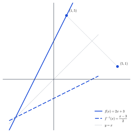
Figure 2.5 — and , from the example of §3, reflected in . The point corresponds to .
The reversibility studied in this section can be read as a question about information. If describes a process that transforms a cause into an effect , the existence of asks whether the effect retains enough information to reconstruct the cause. When is not injective, like , which treats and the same, the effect has irrecoverably lost the sign: two different causes led to the same effect, and no procedure can afterwards tell which one occurred. Injectivity is not, then, merely a technical condition for defining : it is the statement that the process discards no information along the way. A question remains open: whether this idea, that of processes that preserve all the information of their input as opposed to processes that degrade it irreversibly, reaches other kinds of transformation, mathematical or not.
With reversibility made precise, the chapter turns to one last question about the behavior of a function: no longer whether it can be undone, but where it reaches its highest or lowest values. That is the topic of the next section.
Copyright © 2026 Carlos Dagorret — Licensed under Creative Commons Attribution-NonCommercial-NoDerivatives 4.0 International (CC BY-NC-ND 4.0)