Chapter 3 — Polynomials and Rational Functions
3.1 — Polynomial Functions and Their Graphs
Adding and multiplying is all it takes.
In §2.4 we presented , and as isolated entries of a table, without saying what they have in common. What they have in common is this: all three are obtained by applying to the variable , finitely many times, the two operations that provides by axiom, addition and multiplication. In this section we formalize that observation and study three consequences: the domain, the behavior as grows without bound, and the behavior near a point where the function vanishes.
§1. Definition and elements of a polynomial
Section titled Ҥ1. Definition and elements of a polynomialӤ1.3 introduced the polynomial as an algebraic expression. Here we look at it as what interests us in this chapter: a function from to .
Definition. A polynomial function is a function of the form
where is a nonnegative integer and . The numbers are called coefficients, and the subscript indicates which power of the coefficient belongs to. If , we say that has degree , written , and that is its leading coefficient. The zero polynomial, for all , is left out of this classification: no coefficient singles out in it a term of greatest weight, so we assign it no degree.
The definition speaks of coefficients, and what interests us is the function. A legitimate question remains: if two different expressions defined the same function, could they have different degrees? The answer is no, and we prove it below, in the corollary of §2.
No structural restriction limits the domain. Unlike or in §2.2, adding and multiplying real numbers never produces a forbidden operation, so for every polynomial , without exception. This is the first substantive difference with respect to the catalog of §2.4: where had to exclude a point, no polynomial ever needs to.
The three prototypes we already know are, under this definition, the simplest cases. The function is the polynomial of degree with and . The functions and are those of degree and with a single nonzero coefficient. A constant function , including the constant of §2.4, is a polynomial of degree if , and is the zero polynomial if .
§2. Behavior at the ends of the domain
Section titled “§2. Behavior at the ends of the domain”§2.4 §2 defined what it means for to grow without bound as approaches a point from the right. The question that interests us now is different. No polynomial has a forbidden point to approach; what moves away is itself. §2.4 §3 studied a similar situation with as , and there the result was an approach to a fixed value. For a nonconstant polynomial the opposite happens, and to say so with the same rigor we need a new definition.
Definition. Let be a function defined for all greater than some value. We say that grows without bound as if
We read it like this: for every bound , however large, there is a threshold such that, past that threshold, exceeds . We say that decreases without bound as if the analogous condition holds with in place of . The definitions for are obtained by replacing the hypothesis with .
This definition has the same structure as those of §2.4 §2 and §3. Only the hypothesis that triggers the conclusion changes: here, that exceeds a threshold , instead of falling inside an interval . With it we can prove the central result of this section.
Proposition. Let with and . The behavior of as depends only on the sign of : if , grows without bound; if , decreases without bound. The behavior as depends in addition on the parity of : it coincides with that of if is even, and is reversed if is odd.
Proof. We prove something stronger: for every there is such that, if , then and has the same sign as . The four conclusions of the proposition can be read off from this.
For we factor out the term of highest degree:
Let be the largest of the numbers with . If , since we have , and each summand of other than satisfies . There are summands of that kind, so
Let . If , then , that is, , and therefore . In particular for every .
Now let be arbitrary and take . If , since we have , and since ,
Moreover , so has the sign of . For that sign is the sign of , so if and if . For , the sign of is , and the sign of is that of : it coincides with the case if is even and is the opposite if is odd.
The proposition reduces the behavior at the ends, which has four cases according to the sign of and the parity of , to an immediate reading of the term of highest degree. The rest of the polynomial plays no part in the conclusion: the lower-degree terms, however many they are or however large their coefficients, end up dominated by as soon as is large enough.
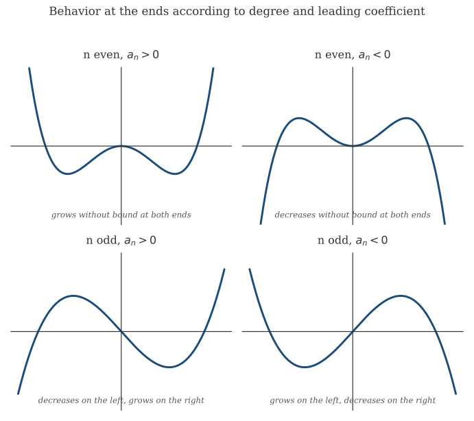 Figure 3.1 — The four possible cases, determined entirely by the sign of and the parity of .
The proposition also has a consequence that settles the question we left open in §1.
Corollary. If two polynomial expressions define the same function, they have the same coefficients. In particular, the degree and the leading coefficient of a polynomial function depend only on the function.
Proof. Let and be two expressions that give the same value for every , and let (padding with zeros any missing coefficients). The function is then identically zero. Suppose some is nonzero and let be the largest index with . If , is the constant , which is not the zero function. If , the proposition applied to gives for sufficiently large, and again is not the zero function. In both cases we reach a contradiction; hence all the are zero, that is, for all .
§3. Multiplicity of a root and its graphical effect
Section titled “§3. Multiplicity of a root and its graphical effect”We say that is a zero or root of if . Let us compare , and at . All three vanish there, but the graph of the first crosses the axis, that of the second touches it and turns back, and that of the third crosses it flattened against it. What distinguishes the three is how many times the factor appears. To say this precisely, we define multiplicity.
Definition. Let be a nonzero polynomial and let . We say that is a zero of of multiplicity if there is a polynomial with such that
For it to make sense to speak of “the” multiplicity we need two things: that the number be determined by and , and that every zero have some multiplicity. We prove the first now.
Proposition. If with and , then .
Proof. Suppose . Subtracting and factoring out gives . By §1.3 §2, for nonzero polynomials; in particular, a product of nonzero polynomials is not zero. Since is not zero, the bracket is: . Evaluating at we obtain , which contradicts . The case is symmetric, so .
The second thing, that every zero of a nonzero polynomial has a multiplicity, is a consequence of the Factor Theorem: each time we extract a factor the degree drops by one, so the process cannot continue indefinitely [Proved in §3.2].
The multiplicity determines how the graph of behaves near . To prove it we first need a result about polynomials that do not vanish at a point: they keep their sign in a neighborhood of that point.
Lemma (sign preservation). Let be a polynomial and with . There exists such that, for every with , has the same sign as .
Proof. We write . For the following identity holds:
which generalizes the difference of squares and the difference of cubes of §1.3. It is verified by distributing: the product is , and the terms of the two sums cancel in pairs, except the first of the first sum, , and the last of the second, .
Suppose . Then , and each of the terms of the preceding sum satisfies . Hence , and summing over ,
Take . If , then . If , this gives ; if , it gives . In both cases has the sign of .
Proposition. Let be a zero of with multiplicity . If is odd, changes sign at : the graph crosses the -axis. If is even, does not change sign at : the graph touches the -axis and returns to the same side.
Proof. Let with . By the lemma, there is such that has on the constant sign of . For in that interval with , the sign of is the product of the sign of and that of . If is even, , so keeps the sign of on both sides of . If is odd, has the sign of : it is negative to the left of and positive to the right, so changes sign.
The case , the simple root, is the most frequent and the easiest to visualize: the graph crosses the axis cleanly. The case is the one that already appeared, unnamed, in of §2.4: the graph touches the axis at and returns to the same sign. Higher multiplicities repeat one of these two patterns, crossing if is odd and tangency if is even. To the eye, the graph flattens against the axis the more, the larger is; that is a visual impression, and what we have proved is only the behavior of the sign.
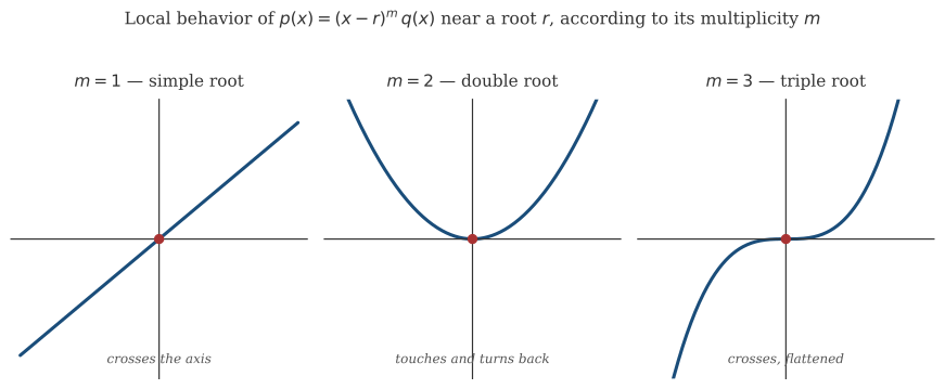 Figure 3.2 — Local behavior near for , and : crossing, tangency, flattened crossing.
In this way we have gathered, for the polynomial in general, the three elements that already organized the study of each prototype in §2.4: the domain, which here has no restriction at all; the behavior at the ends, governed entirely by the term of highest degree; and the local behavior at the points where the function vanishes, governed by the multiplicity. One problem remains, the most elementary of all, which this section postponed on purpose: given a concrete polynomial, how do we effectively determine what its real zeros are? That is the subject of the next section.
Copyright © 2026 Carlos Dagorret — Licensed under Creative Commons Attribution-NonCommercial-NoDerivatives 4.0 International (CC BY-NC-ND 4.0)