Chapter 5 — Trigonometric Functions of Real Numbers
5.4 - Trigonometric Graphs
Every property visible in the graph of a trigonometric function —where it rises, where it falls, where it shoots off to infinity— is already proved in §5.3, or is proved in two more steps from there. This section adds no new behavior: it translates it into an image.
§1. A bounding lemma
Section titled “§1. A bounding lemma”Before being able to prove that shoots off without bound near , a tool is needed that §5.3 did not need: a quantitative bound on how much and can change when changes little. The construction of §5.2 provides it directly.
Lemma. For with , and .
Proof. The difference between two coordinates of two points of the plane never exceeds the Euclidean distance between those points: —distance between and —. That distance, in turn, is the length of the chord joining with , and a chord never exceeds the arc it subtends —§5.1 §2, the chord is, itself, an inscribed approximation of a single segment—. That arc, by the additivity of arc length throughout the construction of §5.2 §1–§3, measures exactly . Chaining the three inequalities, . The same argument, exchanging which coordinate is isolated, gives .
One more symmetry is missing: what relation bears to . From it follows, among other things, that tangent and cotangent have period , half that of sine and cosine. It is the content of §2.
§2. Central symmetry and the period of the tangent
Section titled “§2. Central symmetry and the period of the tangent”Proposition. for all ; equivalently, and .
Proof. The rotation by about the origin —— is an isometry that fixes the center of the circle, sends to , and preserves the length of any arc —being an isometry, it preserves all distances, hence it preserves the perimeters of the inscribed and circumscribed polygons that approximate any arc—. The initial square of §5.1 is symmetric with respect to that rotation —, —, and consequently so is the whole construction by bisection of §5.1 and of §5.2, level by level. Traveling an arc of length from —the rotated point— is, then, the rotated image of traveling an arc of length from ; and since , traveling additional from there reaches . Hence is the rotation of , that is, .
Corollary (period of tangent and cotangent). and , wherever both are defined.
Proof. . Analogous for .
With the tools already gathered, it remains to describe how to read the circular motion of as an ordinary Cartesian graph. It is the content of §3.
§3. From the circle to the graph
Section titled “§3. From the circle to the graph”describes a point that moves on the unit circle as travels through . Graphing or in the - plane is “unrolling” that motion: instead of following the point on the circle, one follows only its height —or its abscissa— as advances along a horizontal line. Each complete turn of —each increment of by — corresponds, in the unrolled graph, to a stretch identical to the previous one, shifted horizontally by : it is the periodicity of §5.3 §4, seen as visual repetition instead of as algebraic equality.
§4. Graphs of sine and cosine
Section titled “§4. Graphs of sine and cosine”The features of the graph of —and, by the same argument, that of — are already, all of them, proved in §5.3: period (§5.3 §4), range attained without exception (§5.3 §3), parity — odd, even— (§5.3 §5), and the exact values at (§5.3 §9). The graph of is, moreover, that of shifted —a consequence that is proved in §5.5, not in this section—.
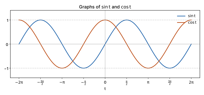 Figure 5.1 — and on . The dotted lines at mark the range; the zero crossings of one coincide with the extrema of the other —a consequence of the Pythagorean identity of §5.3 §2: if , then —.
Tangent and cotangent require a piece that sine and cosine did not need: a proof that, near the points excluded from their domain, the function shoots off without bound. That is where the Lemma of §1 does its work. It is the content of §5.
§5. Graphs of tangent and cotangent
Section titled “§5. Graphs of tangent and cotangent”Proposition (vertical asymptote of at ). For every there exists such that .
Proof. By the Lemma of §1 with , : —using —, and . For , we have . Given , let . If , then , and , so that
The same Lemma, applied from the other side and at each of the points , gives the symmetric behavior — when approaching from the right—, and an identical argument for gives its asymptotes at , where .
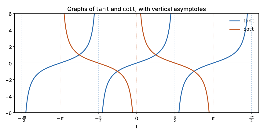 Figure 5.2 — and . The period of both is —Corollary of §2—, half that of sine and cosine; the asymptotes of (longer dashed lines) are where , and those of (dotted lines) where .
Secant and cosecant, being reciprocals of cosine and of sine, inherit their asymptotes exactly where the denominator vanishes —without the need for an additional proof—. It is the content of §6.
§6. Graphs of secant and cosecant
Section titled “§6. Graphs of secant and cosecant”Since , the Proposition of §5 —with the roles of numerator and denominator now inverted, exactly when , which was already proved within that same proof— gives the same vertical asymptotes as , at the same points . Similarly, shares the asymptotes of , at . Unlike tangent and cotangent, however, the period of and of is —that of and , respectively—, not : the Proposition of §2 gave , which changes sign, so that in general.
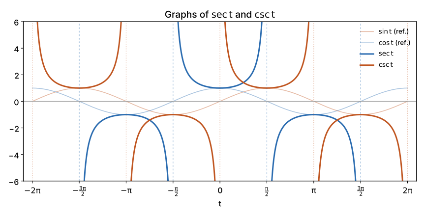 Figure 5.3 — and , with and superimposed in faint stroke as a reference. Where the reference curve approaches , the reciprocal shoots off; where the reference one equals , the reciprocal does too, since .
§7. Worked exercises
Section titled “§7. Worked exercises”Exercise 1. At which points of the interval does have a vertical asymptote?
Solution. By §5.3 §7, excludes the points where ; by §5.3 §9 and the sign table of §5.3 §6, those points are and .
Exercise 2. Using the period proved in §2, compute from .
Solution. Since , the Corollary of §2 gives , and by Exercise 1 of §5.3 §10, . Hence .
Exercise 3. Why does the graph of never take values in ?
Solution. Since for all —§5.3 §3—, and in , we have , whence . Hence , never in the open interval — visible in Figure 5.3, where both branches of always stay at a distance of at least from the horizontal axis.
§8. Close
Section titled “§8. Close”The three graphs of this section —sine with cosine, tangent with cotangent, secant with cosecant— introduced no behavior that §5.3 had not already proved, except for the vertical asymptote of the four unbounded functions, and even that asymptote was proved with a single new tool —the bounding Lemma of §1— applied four times. It is, once again, the pattern that this book pursues from the first chapter: to construct a single piece of machinery with care, and let it reappear as many times as necessary, instead of fabricating a different tool for each occasion.
What remains, to close the chapter, is to see what happens when these six graphs are transformed —shifted, stretched, changing period or amplitude—, exactly as §2.5 did with the catalog of prototype functions of §2.4.
§5.5 applies to the trigonometric functions the same transformations —shift, reflection, change of scale— already studied in §2.5, with a novelty proper to this family: the change of period.
Copyright © 2026 Carlos Dagorret — Licensed under Creative Commons Attribution-NonCommercial-NoDerivatives 4.0 International (CC BY-NC-ND 4.0)