Chapter 2 — Functions
2.3 — Visualization and Basic Topology in the Plane: Global Behavior
A graph is not looked at: it is read, as any other mathematical statement is read.
In §2.1 the graph of a function was defined as a precise subset of , not as an intuitive sketch. This section takes advantage of that precision. Each geometric property we are going to discuss, such as meeting a vertical line, touching the -axis, being symmetric, or going up and down, is an algebraic property translated into the language of the plane, and each can be checked exactly from the formula, without relying on a visual impression.
§1. The vertical line test
Section titled “§1. The vertical line test”At the close of §2.1 a question was left pending: given an arbitrary subset of the plane, how can we recognize whether it is the graph of some function? The answer is a direct translation of the existence and uniqueness conditions of §2.1.
Proposition (vertical line test). Let and . Then is the graph of a function if and only if each vertical line , with , meets in exactly one point.
Proof. The vertical line is the set , and a point of lies on it exactly when its first coordinate is . Suppose that for a function . For each , the points of with first coordinate are the pairs ; by existence there is at least one, and by uniqueness there is at most one. The line therefore meets in exactly one point, . Conversely, suppose that each line with meets in exactly one point. Since , is a relation from to ; having at least one point on each line is existence, and having at most one is uniqueness. Therefore is a function from to , and it is its own graph.
The test adds no new fact: it is the definition of function of §2.1 seen in the plane. That is why the circle of §2.1 fails the test exactly where it failed the definition: each vertical line with meets it in two points, one with and another with .
§2. Domain and image read from the graph
Section titled “§2. Domain and image read from the graph”The domain and the image, defined in §2.1 and computed in §2.2, have a direct geometric reading as projections of the graph onto the axes. The domain is the set of abscissas for which the vertical line touches the graph. The image is the set of ordinates for which the horizontal line touches the graph in at least one point. This reading serves as a quick check, in the spirit of §1.9, but it does not replace the computation of §2.2: a finite window may hide parts of the domain or the image that extend beyond what the screen shows.
It is worth reviewing visually the notation with which domains and images are described: the open and closed intervals of §1.1 and the neighborhood , also from §1.1, which will reappear in §2.4 and in the relative extrema of §2.8.
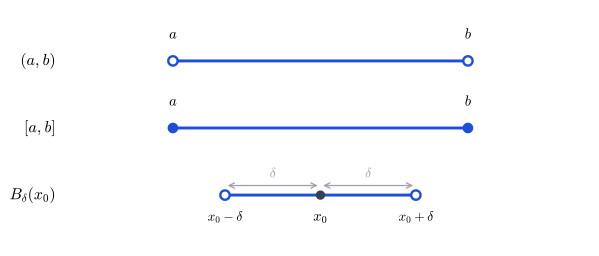
Figure 2.1 — Open interval, closed interval, and neighborhood .
§3. Zeros and sign
Section titled “§3. Zeros and sign”A zero of is a value such that ; geometrically, a point where the graph touches or crosses the -axis. Finding the zeros of a function means solving the equation with the techniques of §1.5.
To know the sign of a function between its zeros, the method is the sign analysis of §1.7. When is a polynomial or a quotient of polynomials, the numerator and the denominator are factored, and the roots of all the factors divide the domain into intervals on which no factor changes sign; therefore neither does . Note that the roots of the denominator matter even though they are not zeros of : has no zero and yet it is negative for and positive for . The sign of a function can change at a point excluded from the domain.
Does the same hold for every function? Not without more. A piecewise function can jump from a negative value to a positive one without passing through zero; for example, the one that equals for and for . For the sign to change only at a zero, the function must have no jumps, a property called continuity, and proving that the sign then changes only at zeros requires a theorem of Calculus, the intermediate value theorem. In this book we apply sign analysis to functions whose expression can be factored, where the argument of §1.7 is complete.
Example. Let . Its only zero is , and its domain excludes . By §1.7, is positive on , negative on and positive on : it changes sign at the zero and also at the excluded point .
§4. Symmetry: even and odd functions
Section titled “§4. Symmetry: even and odd functions”Two kinds of symmetry of the graph deserve a name of their own, because they simplify the study of a function: it is enough to know its behavior for to deduce the rest.
Definition. Let be a function whose domain is symmetric with respect to the origin, that is, . We say that is even if for all , and odd if for all .
The requirement on the domain is not incidental: without it, might not be defined even though is, and the comparison would lose its meaning before it began.
Each of these conditions is the translation of a symmetry from §1.8. If is even, each point of the graph comes with , which is symmetry with respect to the -axis. If is odd, each point comes with , which is symmetry with respect to the origin. The third symmetry of §1.8, with respect to the -axis, is impossible for a function that is not identically zero: if , the symmetry would require to lie on the graph as well, and would have two different values at the same , against the uniqueness of §2.1.
Examples. The function is even, because . The function is odd, because . Most functions are neither even nor odd. For , for example, and : since , it is not even, and since , it is not odd. A single pair of values is enough to rule out both symmetries. Parity is a special property, not the usual situation.
§5. Monotonicity: increasing and decreasing
Section titled “§5. Monotonicity: increasing and decreasing”The last property of this section describes precisely something the graph suggests informally: whether a function goes up or down as advances.
Definition. Let be a function and an interval. We say that is increasing on if for all
and decreasing on if, under the same hypothesis, . If the inequality in the conclusion is non-strict, or , we speak of a nondecreasing or nonincreasing function, respectively. In this book, “increasing” and “decreasing” without qualification refer to the strict case.
The definition does not depend on looking at the graph, but on comparing values of at pairs of points, and that is why it can be checked algebraically without drawing anything. Determining the intervals of monotonicity of functions more complicated than those of this chapter is one of the problems that motivate differential Calculus; here, direct comparison from the definition is enough.
Example. The function is decreasing on and increasing on . We use the lemma of §1.2: if , then . If , the lemma gives directly. If , multiplying by gives , and the lemma gives , that is, . The point belongs to both intervals: there the function finishes decreasing and starts increasing.
The properties gathered in this section, the vertical line test, zeros and sign, symmetry and monotonicity, share a pattern: none is an observation about the drawing, but an algebraic statement that translates exactly into a geometric feature. The graph is useful precisely because that translation exists and is faithful; not because it replaces algebra, but because it makes it visible.
With this vocabulary available, it is time to apply it to a concrete, small set of functions, the elementary prototypes of the chapter, and to study in one of them the behavior near the edges of its domain. That is the topic of the next section.
Copyright © 2026 Carlos Dagorret — Licensed under Creative Commons Attribution-NonCommercial-NoDerivatives 4.0 International (CC BY-NC-ND 4.0)