Chapter 1 — Fundamental Concepts
1.7 — Inequalities
An equation asks where two expressions coincide; an inequality, where one exceeds the other.
An equation looks for the values at which two expressions are equal. An inequality looks for the values at which one is greater or less than the other. It is written with one of the signs , , or between two expressions, and its solution set is, as in §1.5, the set of values of the variable that make it true. The difference lies in the shape of the answer: the solution set of an inequality is usually not a handful of points but an interval or a union of intervals, and the interval notation of §1.1 is the natural way to write it.
The question that guided §1.5 returns here: which steps preserve the solution set. The answer is similar, with one important difference that is worth proving and not merely remembering.
§1. Linear inequalities
Section titled “§1. Linear inequalities”The order axioms of §1.1 say that if , then for every real , and for every . Adding the same number to both sides, or multiplying them by the same positive number, preserves the direction of the inequality. Both steps can be undone, by adding or multiplying by , which is also positive, as we will see shortly. They therefore yield equivalent inequalities, in the same sense as in §1.5. With a negative number, on the other hand, the direction is reversed.
Proposition. If and , then .
Proof. Since , adding to both sides gives . Since , also . The product of two positive numbers is positive, so , that is, . Adding to both sides, .
Dividing by is multiplying by , and has the same sign as : since , and the product of two numbers of opposite sign is negative, and cannot have opposite signs. That is why dividing by a positive number preserves the direction and dividing by a negative one reverses it. The reversal is not a typographical convention: it is a consequence of how the negative reals are ordered, and it will reappear in the rest of the section whenever the sign of a factor is unknown.
Example. Let us solve . Adding leaves . Multiplying by , which is negative, reverses the direction: . The solution set is . Let us check with one value: for , is true, and indeed .
§2. Polynomial inequalities
Section titled “§2. Polynomial inequalities”An inequality such as is not solved by isolating , because there is no step that leaves alone on one side. It is solved by a sign analysis, which rests on the factoring of §1.3. The idea is that the sign of a product depends only on the signs of its factors: by the order axioms of §1.1, a product of nonzero reals is positive if the number of negative factors is even, and negative if it is odd; and by the zero product property of §1.5, it is zero if and only if some factor is.
The procedure is as follows. We bring the inequality to the form , or , or with or , leaving zero on one side. We factor completely over . Each factor has a sign that is easy to know. A linear factor is positive if and negative if . An irreducible quadratic factor , with , always has the sign of : in the proof in §1.3 we wrote it as times a positive quantity. The roots of the linear factors divide the line into intervals, and within each interval no factor changes sign, so neither does the product. It suffices to determine the sign of the product on each interval and choose those that satisfy the inequality, adding the roots when the inequality is or .
Example. Let us solve . Factoring, . The roots and divide the line into three intervals: , and . On the first, both factors are negative and the product is positive. On the second, is positive and negative, and the product is negative. On the third, both are positive and the product is positive. Since the inequality is strict, the roots are not included. The solution set is , where is the union of sets from §1.1.
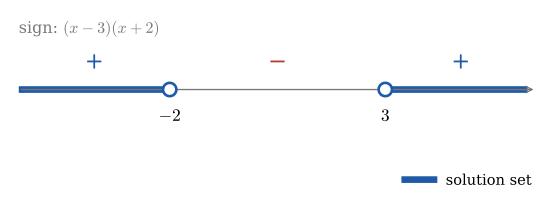
Figure 1.2 — Sign analysis of : the highlighted regions are the solution set.
A repeated factor deserves attention. In , the factor is a square, positive except at , where it is zero; it does not change sign when passing through . The sign of the product is therefore that of , except at , and the solution set is . The rule that the sign “alternates” from one interval to the next holds only when each root appears once.
§3. Absolute value inequalities
Section titled “§3. Absolute value inequalities”These inequalities are solved by translating them into inequalities without absolute value. The translation rests on a lemma that follows from the definition of absolute value in §1.1 and has a geometric reading: is the distance between and .
Lemma. Let and . Then:
(i) if and only if ;
(ii) if and only if or .
Proof. We separate two cases according to the sign of . If , then , and moreover ; therefore is equivalent to , which is equivalent to , and is equivalent to , because is impossible. If , then , and moreover ; by the proposition of §1, is equivalent to , and is equivalent to . In both cases we obtain (i) and (ii).
With and in place of and , the same proof gives the non-strict versions. The hypothesis matters: if , the inequality has no solution, because an absolute value is never negative.
Applying the lemma to , the inequality says that is less than away from :
that is, , which is the neighborhood of of radius from §1.1. The opposite inequality, , says that is more than away from , which happens on both sides of the point:
The difference in shape between the two cases, a bounded interval for "" and a union of two unbounded intervals for "", is no accident. It is the difference between being near a point, which happens only in a limited region around it, and being far from it, which happens everywhere outside.
Example. Let us solve . By the non-strict version of the lemma, it is equivalent to . Adding , , and multiplying by , which is positive, . The solution set is .
§4. Rational inequalities
Section titled “§4. Rational inequalities”A rational inequality, such as , is solved with the same sign analysis as in §2, applied to the numerator and the denominator. The justification is that and, as we saw in §1, has the same sign as ; the sign of the quotient is therefore the one the product would have.
What must not be done is to multiply both sides by the denominator. Its sign depends on , and the proposition of §1 says that, according as it is positive or negative, the direction is preserved or reversed. Multiplying without knowing which of the two cases occurs produces wrong results. For example, from one might “deduce”, multiplying by , that ; but satisfies the original inequality, because , and does not satisfy . The correct course is to leave zero on one side: , whose sign analysis gives the solution set .
The procedure, then, brings everything to one side and leaves zero on the other, factors numerator and denominator, and analyzes the sign of the quotient on each interval determined by all the roots, those of the numerator and those of the denominator. The roots of the denominator are always excluded, whatever the sign of the inequality, because by §1.4 they do not belong to the domain of the expression.
Example. Let us solve . The roots that matter are , from the numerator, and , from the denominator, which is excluded. On the numerator and the denominator are negative, and the quotient is positive. On the numerator is negative and the denominator positive, and the quotient is negative. On both are positive, and the quotient is positive. The inequality asks for negative values or zero: we take the interval and the point , where the quotient is zero and which does belong to the domain, but never . The solution set is .
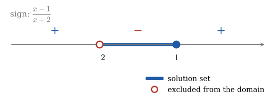
Figure 1.3 — Sign analysis of : is excluded from the domain (red circle) even though the inequality is ""; is included (filled blue circle).
With equations and inequalities solved on the real line, the chapter moves to the plane: the analytic geometry of the next section translates these same algebraic ideas into the language of points, distances and curves.
Copyright © 2026 Carlos Dagorret — Licensed under Creative Commons Attribution-NonCommercial-NoDerivatives 4.0 International (CC BY-NC-ND 4.0)