Chapter 3 — Polynomials and Rational Functions
3.5 — Rational Functions
Where the polynomial never forbade anything, the quotient forbids exactly where the denominator vanishes.
§3.1 opened the chapter by noting that adding and multiplying exhausts the construction of the polynomial. The fourth operation of , division, is still missing, and applying it to two polynomials produces a rational function: , with polynomials and not the zero polynomial. Unlike or separately, inherits from division the same restriction that already imposed in §2.2: there are points where is, quite simply, not defined.
§1. Definition and domain
Section titled “§1. Definition and domain”Definition. A rational function is , where and are polynomials and is not the zero polynomial. Its domain is
By §3.2, has at most finitely many real zeros, at most , so that excludes, at most, finitely many points of : never a whole interval, unlike what would happen if could vanish over a continuous range. This observation, trivial in appearance, is what guarantees that it is worth asking, as the rest of this section does, what happens near each of those excluded points: they are isolated points, surrounded by values where is defined.
§2. Near a zero of the denominator: holes and vertical asymptotes
Section titled “§2. Near a zero of the denominator: holes and vertical asymptotes”A zero of does not always produce the same phenomenon. The difference depends on whether that same value also annuls , and with what multiplicity, the concept already formalized in §3.1 and extended in §3.4.
§2.4 formalized what it means for a function to grow without bound near an excluded point, but it did not formalize the case in which, instead, it stabilizes at a finite value near that point; it only did so for . We need that counterpart, now for a finite point.
Definition. Let be a function defined in a neighborhood of , except possibly at . We say that approaches a real number as if
This definition reuses, unaltered, the distance inequality already fixed in §2.4 §3; the only thing that changes is the hypothesis that activates it, , a neighborhood of a finite point, with that point explicitly excluded, in place of .
Proposition. Let be a zero of of multiplicity , and let be the multiplicity of as a root of ( if ). Then:
(a) if , approaches a real number as ; is a hole of ;
(b) if , the line is a vertical asymptote of .
Proof. By the complete factorization of §3.4, write and , with and . For ,
Case . The exponent , so that is a polynomial well defined at , and is defined in a neighborhood of , since . Let if , or if ; in both cases, the continuity of the algebraic operations on real numbers (sum, product and quotient by something nonzero, already used without naming it in §3.1 §3) guarantees that, given , there exists such that forces . The explicit proof repeats, coordinate by coordinate, the same kind of bounding already practiced in §3.1 §2, and it is omitted because it is mechanical.
Case . The exponent , so that with . Since is a fixed nonzero real number, behaves, near , like a nonzero constant divided by , exactly the situation of near already resolved in §2.4 §2, except for a multiplicative constant and, possibly, a power greater than one: the same argument as in that proposition, adapted by that constant, shows that grows without bound as , and therefore so does or on each side, according to the signs of and of . The line is, by definition, a vertical asymptote.
The case deserves a final clarification: although approaches , the point remains excluded from , since the definition of as a quotient excludes it by construction, regardless of the fact that was indeed defined there. That is, precisely, the phenomenon that informal vocabulary calls a hole: a single missing point in a graph that would otherwise be a continuous curve.
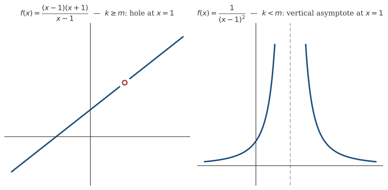
Left: , hole. Right: , vertical asymptote.
§3. Behavior at the ends: the horizontal asymptote
Section titled “§3. Behavior at the ends: the horizontal asymptote”The question of interest now is the same one that organized §3.1 §2 for polynomials: what happens when itself grows without bound. But the result, for a quotient, is different in nature: it does not always grow without bound as every nonconstant polynomial did.
Proposition. Let with and .
(a) If , approaches as , and also as .
(b) If , approaches , the quotient of the leading coefficients, as .
(c) If , has no horizontal asymptote: grows without bound.
Proof. Factor, as in §3.1 §2, and , where and are sums of terms that can be bounded arbitrarily close to as , exactly as was proved in that section. Then, for sufficiently large in absolute value,
and the second factor approaches as , by the same bounding argument of §3.1 §2 applied to and separately. All the behavior of is then governed by : if , the exponent is negative and , giving case (a); if , the exponent is and the factor is the constant , giving case (b) directly; if , the exponent is positive and grows without bound, by the same proposition of §3.1 §2, giving case (c). In each case, translating “the second factor approaches ” into the corresponding - or - definition completes the formal proof, with the same kind of bounding already practiced repeatedly.
§4. Oblique asymptote
Section titled “§4. Oblique asymptote”One case remains that the proposition of §3 declared, without developing it, “without horizontal asymptote”: . Within that case there is one that is particularly orderly, , where does not stabilize at a horizontal line, but does stabilize at a line with slope.
Definition. The line is an oblique asymptote of if approaches as , in the sense of §2 of this section, with .
Proposition. If , has an oblique asymptote.
Proof. By the division algorithm of §3.2, there exist unique and such that , with . Since , the quotient has degree exactly : write . Dividing the identity by ,
so that . Since , case (a) of the proposition of §3, applied to in place of , guarantees that approaches as . Hence approaches , and is an oblique asymptote by definition.
The construction is, in essence, the same division that already organized §3.2 completely: the oblique asymptote is not a new phenomenon in its mechanics, but the reappearance of the division algorithm proved there, now read from the perspective of behavior at infinity instead of the search for roots. And it is, by construction, mutually exclusive with the horizontal asymptote: a rational function has one or the other, never both, because the case of §4 and the cases of §3 are disjoint.
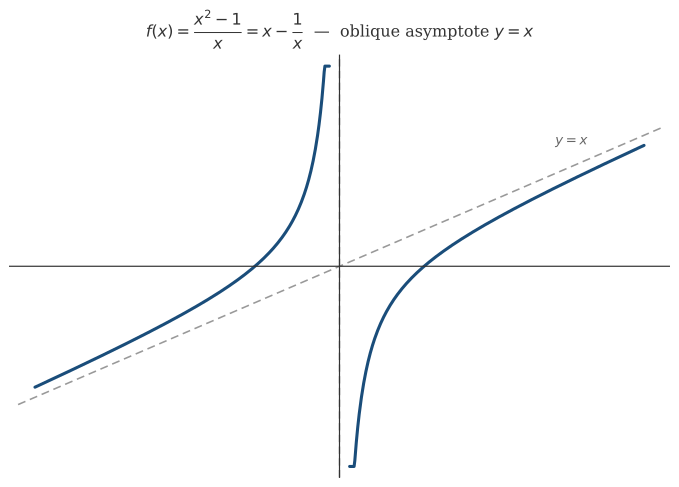
: the term vanishes, leaving the line .
With domain, holes, and vertical, horizontal and oblique asymptotes already completely characterized, the catalog of possible behavior of a rational function is closed. That closure is not merely technical: it is also, in a broader sense, the closure of the question that opened this chapter in its index, about what it means to construct, and not simply to enumerate, the mathematical objects one works with. That reflection, more philosophical than algebraic, is the subject of the final section of the chapter.
Copyright © 2026 Carlos Dagorret — Licensed under Creative Commons Attribution-NonCommercial-NoDerivatives 4.0 International (CC BY-NC-ND 4.0)